Once upon a time I considered becoming a meteorologist. I was the kind of kid who was always outside and much to my mom’s dismay, this included running out into the rain. Creek walking, as we called it, was a thing we did and when the water rose, so did our hopes of rafting down it.
You can imagine my mom’s joy as I survived childhood mostly intact, only to learn that when I was old enough to sign the waiver, I did my first skydive. A new appreciation of weather was born. Skydiving through falling rain hurts you know. As fate would have it, I also began my career in software development at that time.
In 2005 I had the great pleasure of joining the weather branch of Universal Weather and Aviation as a software developer. Then called ImpactWeather, I spent nearly 15 years exploring the weather through technology. Now part of StormGeo, ImpactWeather may be in the past, but I still have one eye on the weather – and a lot more experience creating tools to plan my next creek walking adventure. Follow along as I create a radar map for a new project at stormlio.com.
Overview
I am going to show you how to create your own weather radar images using readily available data and tools. The goal is to prototype one straight forward, end-to-end method of achieving this. I think each component of this prototype could have it’s own article. However, I’ll start by hitting the high notes in order to see it through. The result will be a fully functional radar map, and you will learn some techniques for exploring weather data for your own adventures.
The Radar Data
There are a variety of radar data sets to choose from. Within each of these data sets are a multitude of products designed for different purposes. For example, when a radar ground station is collecting data, it scans horizontally and tilts vertically as it rotates. There are data sets available for each of the tilts as well as a composite of them all. The data set we will use here is the Multi-Radar Multi-Sensor (MRMS) 2D composite reflectivity product provided by NOAA that has been quality controlled to remove false echoes and other artifacts.
The data comes as GZIP compressed files that are in the GRIB version 2 file format. In my experience, the grib2 file format can be hit or miss when finding tools that understand its nuances. This can also vary between data sources. Fortunately, the MRMS data set can be processed with GDAL. This is what I will focus on here.
The Development Environment
The GDAL toolset is extremely useful, but it can be a beast because it does so many things. You will have to set up your environment and make sure it is sane before you can process the GRIB2 data.
For this example, I will use the GDAL libraries available in Python. I chose this method over GDAL command line tools because we can perform all the steps necessary to create the raster images with GDAL in one shot without cluttering everything up with a lot of temporary files and other housekeeping tasks.
Whether you choose to use a python virtual environment, a Docker container, or just install the needed libraries this will be a prerequisite task for you. This example uses the requests library and the GDAL library. Although the generated requirements.txt states you need osgeo, which seems to be dummy library.
requests==2.31.0
osgeo==0.0.1
The script below is our starting point. This will reasonably test that your environment is sane before moving on.
#!/usr/bin/python3

from pprint import pprint
from osgeo import gdal, gdalconst

def main():
    source_url = ('https://mrms.ncep.noaa.gov'
        '/data/2D/MergedReflectivityQCComposite/'
        'MRMS_MergedReflectivityQCComposite.latest.grib2.gz')


    ds = gdal.Open(f'/vsigzip//vsicurl/{source_url}')
    meta = ds.GetRasterBand(1).GetMetadata()
    ds = None

    pprint(meta);

if __name__ == '__main__':
    main()
If everything is ready to proceed, you should see output similar to the following after running this script.
{'GRIB_COMMENT': 'Composite Reflectivity Mosaic (optimal method) [dBZ]',
 'GRIB_DISCIPLINE': '209',
 'GRIB_ELEMENT': 'MergedReflectivityQCComposite',
 'GRIB_FORECAST_SECONDS': '0',
 'GRIB_IDS': 'CENTER=161(US-OAR) SUBCENTER=0 MASTER_TABLE=255 LOCAL_TABLE=1 '
             'SIGNF_REF_TIME=3(Observation_time) REF_TIME=2024-02-05T20:14:37Z '
             'PROD_STATUS=2(Research) TYPE=7(Processed_radar_observations)',
 'GRIB_PDS_PDTN': '0',
 'GRIB_PDS_TEMPLATE_ASSEMBLED_VALUES': '10 0 8 0 97 0 0 0 0 102 0 500 255 1 0',
 'GRIB_PDS_TEMPLATE_NUMBERS': '10 0 8 0 97 0 0 0 0 0 0 0 0 102 0 0 0 1 244 255 '
                              '1 0 0 0 0',
 'GRIB_REF_TIME': '1707164077',
 'GRIB_SHORT_NAME': '500-GPML',
 'GRIB_UNIT': '[dBZ]',
 'GRIB_VALID_TIME': '1707164077'}
About the Map
We are going to be creating radar images and displaying them on a simple map using Leaflet and OpenStreetMap (OSM). As such, once we have the data from the GRIB files, we’ll need to re-project the data into the map projection used by OSM & Leaflet. This is Web Mercator, or more specifically EPSG:3857. If this makes your head spin, don’t worry. Fortunately, GDAL can do this for us too!
gdal.Warp('/vsimem/reprojected.tiff', dstSRS='EPSG:3857', srcDSOrSrcDSTab=ds, resampleAlg=gdalconst.GRA_Average)Adding Color
Now that the data is re-projected, we can prepare for creating the final raster image. This means assigning a color to each of the values in the data set. In this case the unit of measurement used is dBZ. Which is decibel relative to Z.
Here is the color ramp we will use. Note that you define a value in dBZ followed by an RGBA color. With the exception of -99 and -999, other negative values will generally be frozen precipitation. -999 in this data set represents NODATA and -99 shows the bounds of the data. Both of these are transparent in this example.
-999 0:0:0:0
-99 0:0:0:0
75 153:85:201
70 255:0:255
65 192:0:0
60 220:0:0
55 255:0:0
50 255:144:0
45 231:192:0
40 255:255:0
35 0:144:0
30 0:200:0
25 0:255:0
20 0:0:246
15 1:160:246
10 0:236:236
5 119:119:119
0 169:168:125
-5 214:212:173
-10 115:74:119
-15 163:127:167
-20 208:175:212
-25 216:210:233
-30 221:254:255
-35 204:221:221
With the color ramp saved as radar_ramp.txt, we can rasterize the data and apply our colors. No surprise here, GDAL makes this a breeze. Just supply the location of your color ramp. Note that we will be writing the PNG image to latest.png in the current directory.
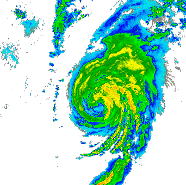
gdal.DEMProcessing('latest.png', ds, 'color-relief', colorFilename="./radar_ramp.txt", format="png", addAlpha="true")This will leave us with a semi transparent PNG image like below. Cool, but not super rad without some point of reference about where we are looking.
Map It
To wrap up the example I’m going to show you how to use Leaflet to display a web based map of our radar. For demonstration purposes we will also be using map background tiles provided by OpenStreetMap.
In order to correctly place our image on a map with Leaflet we need to know where in the world the image should be. This information can be obtained while creating the image, and then we can supply these values to Leaflet when loading the image.
info = gdal.Info(ds, format='json')
print(json.dumps(info['wgs84Extent'], indent=2))
This results in the following GeoJSON
{
  "type": "Polygon",
  "coordinates": [
    [
      [
        -130.0,
        55.0
      ],
      [
        -130.0,
        20.0026826
      ],
      [
        -59.9967935,
        20.0026826
      ],
      [
        -59.9967935,
        55.0
      ],
      [
        -130.0,
        55.0
      ]
    ]
  ]
}
A Front End
From the GeoJSON above we only need two corners, lets use the bottom left and top right. The complete example is below.
<!DOCTYPE html>
<html lang="en">
<head>
<meta charset="utf-8">
<meta name="viewport" content="width=device-width, initial-scale=1">
<title>Example MRMS Composite Reflectivity</title>
<link rel="stylesheet" href="https://unpkg.com/[email protected]/dist/leaflet.css"
integrity="sha256-p4NxAoJBhIIN+hmNHrzRCf9tD/miZyoHS5obTRR9BMY=" crossorigin="" />
<script src="https://unpkg.com/[email protected]/dist/leaflet.js"
integrity="sha256-20nQCchB9co0qIjJZRGuk2/Z9VM+kNiyxNV1lvTlZBo=" crossorigin=""></script>
<style>
html,
body {
margin: 0;
padding: 0;
}
#map {
position: absolute;
top: 0;
bottom: 0;
width: 100%;
}
</style>
</head>
<body>
<div id="map"></div>
<script>
const bounds = [
[20.0026826, -130.0], // bottom left
[55.0, -59.9967935] // top right
];
const map = L.map('map').fitBounds(bounds);
const tiles = L.tileLayer('https://tile.openstreetmap.org/{z}/{x}/{y}.png', {
maxZoom: 19,
attribution: '© <a href="http://www.openstreetmap.org/copyright">OpenStreetMap</a>'
}).addTo(map);
map.whenReady(function () {
L.imageOverlay('./latest.png', bounds, {opacity: 0.5}).addTo(map);
});
</script>
</body>
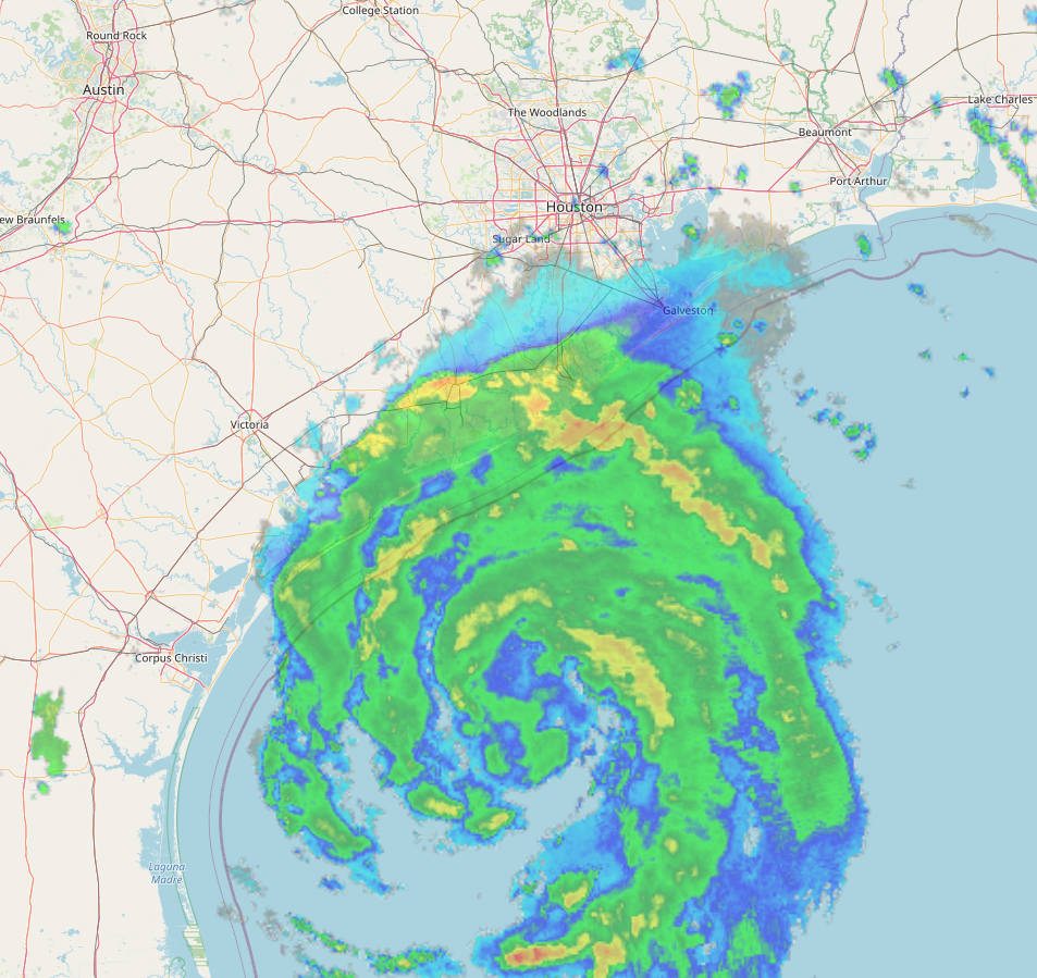
</html>The Result
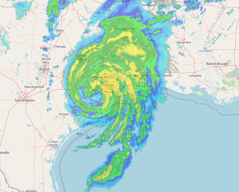
Take Five
Congratulations. We now have a functional radar map that shows the most current radar data. There is a lot more we can do such as animation or updating it with new images. If you would like to see more send me a message.
You can download all the code from this example on GitHub.
More Weather
I am currently working on updating the weather site stormlio.com. Try it out and let me know what you think!